Hello again! It’s time for another blog post. Reaching this great milestone of a second post means two things – I can call myself a blogger without lying (my first step towards fame, I’m certain) and that I have officially stuck to this project for longer than any hobby other than playing videogames. And people say I don’t take things seriously…
In this post, we’re going to talk a little about Deep Learning (DL) and, more specifically, Neural Networks (NNs). I’m aware that last time I promised a more technically focussed post looking at a specific architecture and I did indeed have a post on Siamese Neural Networks (SNNs) mostly written, but it occurred to me that I was glancing over what was actually happening between the nodes. Since the core of this blog is helping those who are interested to understand the nitty gritty details, I decided that we should examine neural networks in a more general context first and move on to some architectural nuances in later posts.
Another reason behind this post is that it’s actually reasonably difficult to find a clear and straightforward description of exactly what’s happening within a neural network. Nick Taylor, a researcher at the Edinburgh Centre for Robotics, recently talked briefly about this during a SICSA AI meet at Stirling University:
“Neural Networks are the focus of much recent work, but are precisely that which results are most difficult to understand and explain.”
This isn’t just a problem for a single PhD student such as myself, but rather an issue which challenges the research community at large. With that in mind, the only way we’re going to get better at dealing with it is by practicing and developing more resources to help ourselves. So without further ado!
… A Quick Introduction to Deep Learning
Deep Learning (DL) is member of a group of machine learning methods which learn the features to extract from input data to develop a new representation of that same data. In many instances, this new representation makes it easier or more efficient to perform traditional machine learning methods such as case-based reasoning and k nearest neighbour [1]. Part of the reasoning behind this is that the newly learned representation is quite flexible, as it is does not suffer from any reliance upon task-specific rules or algorithms which can often cause a lot of trouble if one is using manually-coded features.
Artificial Neural Networks (ANNs) and Deep Neural Networks (DNNs) are particular types of DL algorithm. That said, they are far and away the most popular, and are usually broadly categorised under the singular moniker neural networks, as the difference between them is minor.
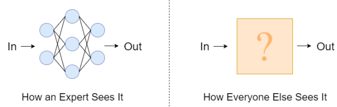
What sets neural networks (and DL algorithms in general) apart from other ML techniquesis the belief that a new data representation can be better learned through a ‘deep’ function than a series of shallow functions. Sounds a bit complex? Well, the easiest way to think about this is to think about a computational graph.
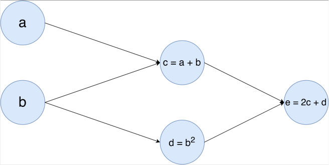
Now for those that haven’t come across these before, computational graphs are just a method to visualise functions whose variables rely upon each other. In the simple example above, we can see that c‘s value is reliant upon a and b while e‘s value is reliant upon c and d.
The easiest way to think about a neural network is to consider a special type of computational graph that has two rules – (1) that each node in one layer is connected to every node in the following layer (though this is not true in every architetcure, we can take it as a rough generalisation for the time being) and (2) the output of each node must be differentiable. Rule (2) is very important in modern neural networks, and we’ll explain why in the next bit.
… Training a Neural Network
Neural networks are really a supervised learning method, as their development requires a set of example data, known as the training set, where the desired output is already known. Training a neural network also makes use of a loss function, backpropagation and an optimization algorithm. Now, we’re not going to examine any of these concepts in too much detail here. Each of these three is more than deserving of its own post, and there are various loss functions and optimizers for various situations to boot, but we will set the scene by offering a quick description of each concept.
Loss Function: A loss function’s job is to calculate the difference between a piece of data’s estimated value and its true value to produce an error value. How does the network know the data’s true value? We tell it – which is why we require a training set where the desired output is already known. There are various loss functions that work better in different situations, but the primary objective always remains the same.
Backpropagation: This is one of those scary concepts that was invented because no one wanted to use the term reverse-mode differentiation – because that is exactly what it is. Now I’m not going to explain the full process (mostly because it is done superbly at this blog by Chris Olah [2]), but it is sufficient to say that backpropagation calculates how each and every node in the network contributes to the error value – and you cannot perform it if your network architecture doesn’t follow rule (2)!
Now, I’m cheating a little bit here – you don’t have to use backpropagation to do this calculation, and there are plenty of instances in older research where researchers didn’t. But in modern neural networks with potentially millions of nodes, the cost of doing this calculation without backpropagation would be enormous – enough so that it would increase your training time by potentially years. See why rule (2) is so important now?
Optimization Algorithm: The optimization algorithm (or optimizer as it is often called) does exactly what it says on the tin; it optimizes the weights and parameters of the nodes of a neural network to minimise the error value. When used in correlation with backpropagation, gradient descent optimizers are most commonly used. Have a look here [3] for a more detailed examination of how they work.
Okay, so let’s put these altogether and walkthrough the process of training a neural network from start to finish.
Data is input to the neural network and is fed through in sequence, with each layer of the network reliant upon the output of the preceding layer. After a piece of data from the training set has been fed through a network, a loss function calculates the difference between the output of the neural network and the desired output. Backpropagation then calculates the error contribution of each node in the network in regards to the output. The weights or parameters of each node are then updated appropriately by the optimizer.
This process is completed for every piece of data in the training set, and is usually repeated over multiple times in order to optimise the nodes. The resultant network can then be applied to data where the desired output is not known and perform its task unsupervised.
And that’s it!
Okay, so that’s a very brief (and hopefully clear) introduction to neural networks – below are a few interesting reads that helped inform this article, for those who are interested. Thank you very much for reading and I hope that HAL will let you all leave with your helmets.
[1] Representation Learning: A Review and New Perspectives – Bengio, Courville and Vincent. 2014.
[2] Calculus on Computational Graphs: Backpropagation – Colah’s Blog. 2015
[3] An Overview of Gradient Descent – Sebastien Ruder’s Blog. 2016